from IPython.display import Image
import matplotlib.pyplot as plt
import xarray as xr
import numpy as np
from tensorflow import keras
from tensorflow.keras.models import load_model1 Introduction
Convincing evidence has shown that air pollution is a major environmental risk to health. The World Health Organization (WHO) estimates that 4.2 million premature deaths occur each year due to outdoor air pollution (Majeed et al. (2024)). In South Asia, air pollution is a major public health concern, with high levels of particulate matter (PM2.5) and other pollutants (Majeed et al. (2024)). Monitoring air quality is essential for public health and environmental protection. Satellites provide a valuable tool for monitoring air quality, as they can measure pollutants such as methane (CH4), nitrogen dioxide (NO2), sulfur dioxide (SO2), carbon monoxide (CO), Formaldehyde (HCHO), and ozone (O3) from space. Using these variables,the Sentinel-5P product also calculates the Aerosol Index (AI) which is a measure of the amount of aerosols in the atmosphere. The AI is used to monitor air quality and can be used to forecast air quality events such as smog. The aerosol index (AI) is a measure of the amount of aerosols in the atmosphere and is used to monitor air quality. The AI data from the Sentinel-5P satellite is available in near real-time and can be used to monitor air quality (ESA (2021)).
In this project, we will use a convolutional LSTM neural network to forecast the AI in South Asia. The goal of this project is to develop a model that can accurately predict the AI in the future and help in monitoring air quality. The convolutional LSTM neural network is a class of neural networks that is used for spatio-temporal data (Shi et al. (2015)). It combines the spatial information from convolutional layers with the temporal information from LSTM layers. The convolutional LSTM neural network has been shown to be effective for predicting spatio-temporal data such as weather forecasting (Kumar et al. (2020)) and anomaly detection (Luo, Liu, and Gao (2017)).
The goal of this project is to develop a model that can accurately forecast the AI in the future and help in monitoring air quality.
In [1]:
2 Data
An arbitary study area was chosen which confined to bounding box covering northern regions of South Asia as these regions continuosly experience some of world’s worst air quality (Majeed et al. (2024)). The bounding box coordinates were:
bbox = [68.137207,24.886436,84.836426,34.379713] #WGS84 // lon,lat,lon,latFor the study area abive, the corresponding Sentinel-5P data was downloaded using the Deep Earth System Data Lab’s xcube sentinel datatore (Brandt (2023)). The attached notebook titled deepesdl-S5PL2.ipynb can be viewed to see how this works. ALternative, the attached script titled data.py as a Code Link in this manuscript document can also be used to download the raw data.
However, for ease, the downloaded version resulting file can be found on Zenodo (Khan (2024)).
The timeperiod for the study was chosen from 01.01.2019 to 31.12.2023. The data was downloaded from the Sentinel-5P data store using the Deep Earth System Data Lab’s xcube sentinel datatore (Brandt (2023)). The data was downloaded in the form of netCDF files which contain the AI data for the study area and time period. The data was then preprocessed and split into training and testing datasets. The training dataset contains the AI data from 01.01.2019 to 31.02.2022 and the testing dataset contains the AI data from 01.01.2023 to 31.12.2023.
The spatial resolution of the data is 3.629km x 3.269km per pixel.
Here is the resulting dataset:
In [2]:
ds = xr.open_dataset('S5PL2_5D.nc')
ds
<xarray.Dataset> Size: 2GB
Dimensions: (time: 366, lat: 291, lon: 512, bnds: 2)
Coordinates:
* lat (lat) float64 2kB 34.36 34.33 34.3 ... 24.97 24.94 24.9
* lon (lon) float64 4kB 68.15 68.19 68.22 ... 84.75 84.79 84.82
* time (time) datetime64[ns] 3kB 2019-01-03T12:00:00 ... 2024-01...
time_bnds (time, bnds) datetime64[ns] 6kB ...
Dimensions without coordinates: bnds
Data variables:
AER_AI_340_380 (time, lat, lon) float32 218MB ...
AER_AI_354_388 (time, lat, lon) float32 218MB ...
CH4 (time, lat, lon) float32 218MB ...
CLOUD_FRACTION (time, lat, lon) float32 218MB ...
CO (time, lat, lon) float32 218MB ...
HCHO (time, lat, lon) float32 218MB ...
NO2 (time, lat, lon) float32 218MB ...
O3 (time, lat, lon) float32 218MB ...
SO2 (time, lat, lon) float32 218MB ...
Attributes:
Conventions: CF-1.7
title: S5PL2 Data Cube Subset
history: [{'program': 'xcube_sh.chunkstore.SentinelHubC...
date_created: 2024-05-02T13:00:01.155492
time_coverage_start: 2019-01-01T00:00:00+00:00
time_coverage_end: 2024-01-05T00:00:00+00:00
time_coverage_duration: P1830DT0H0M0S
time_coverage_resolution: P5DT0H0M0S
geospatial_lon_min: 68.137207
geospatial_lat_min: 24.886436
geospatial_lon_max: 84.836426
geospatial_lat_max: 34.377593673828122.1 Predictor variables (features)
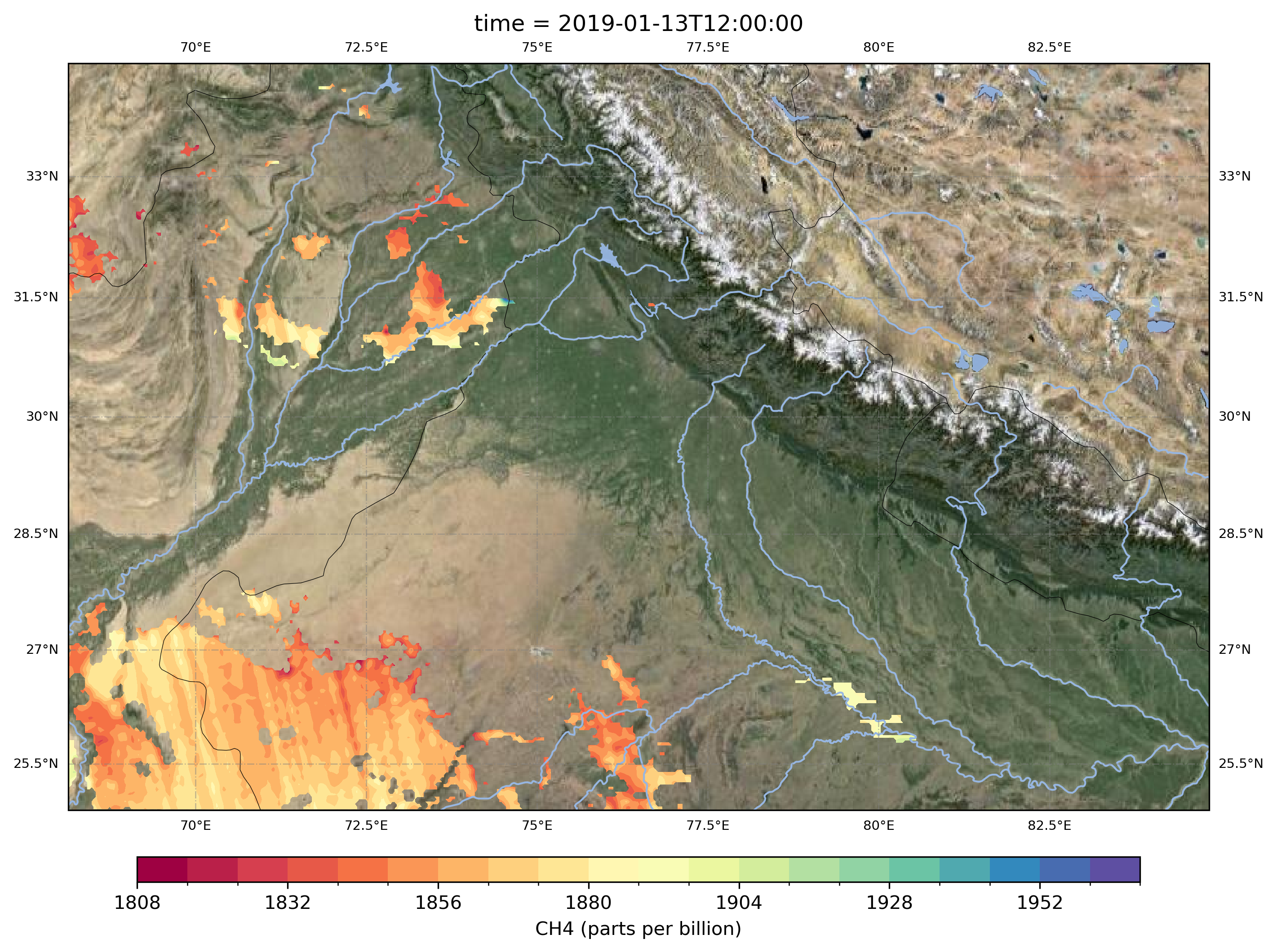
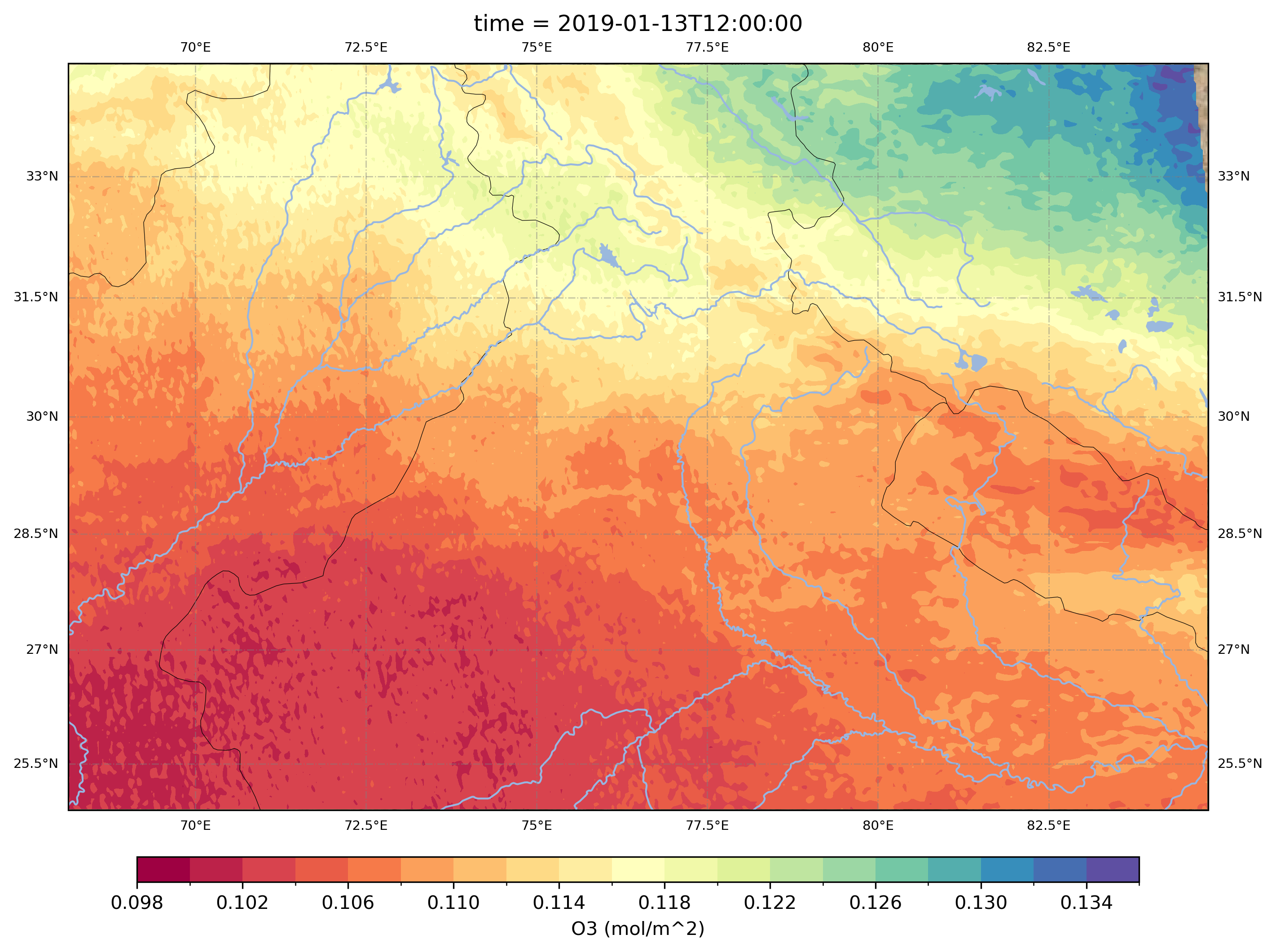
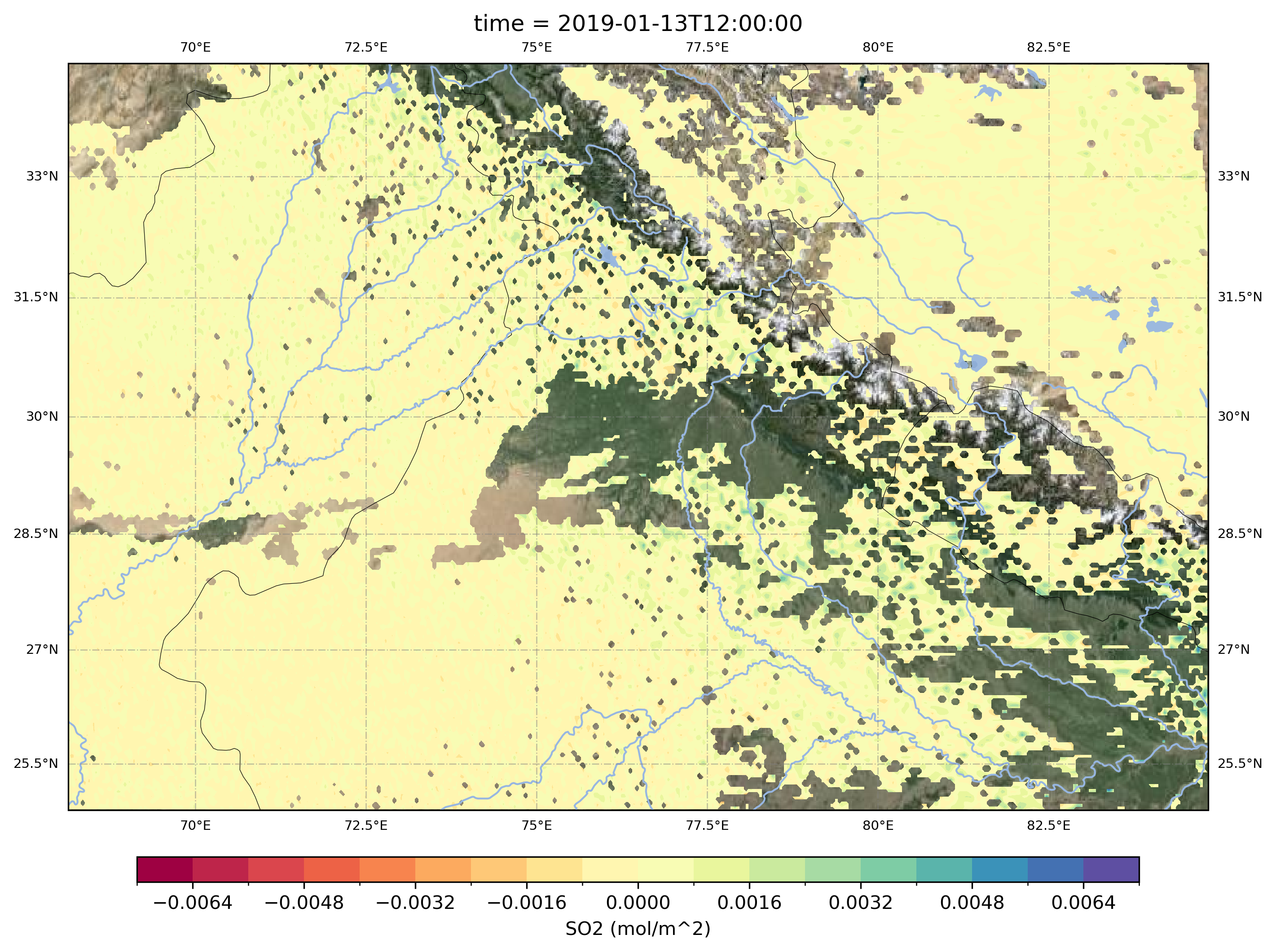
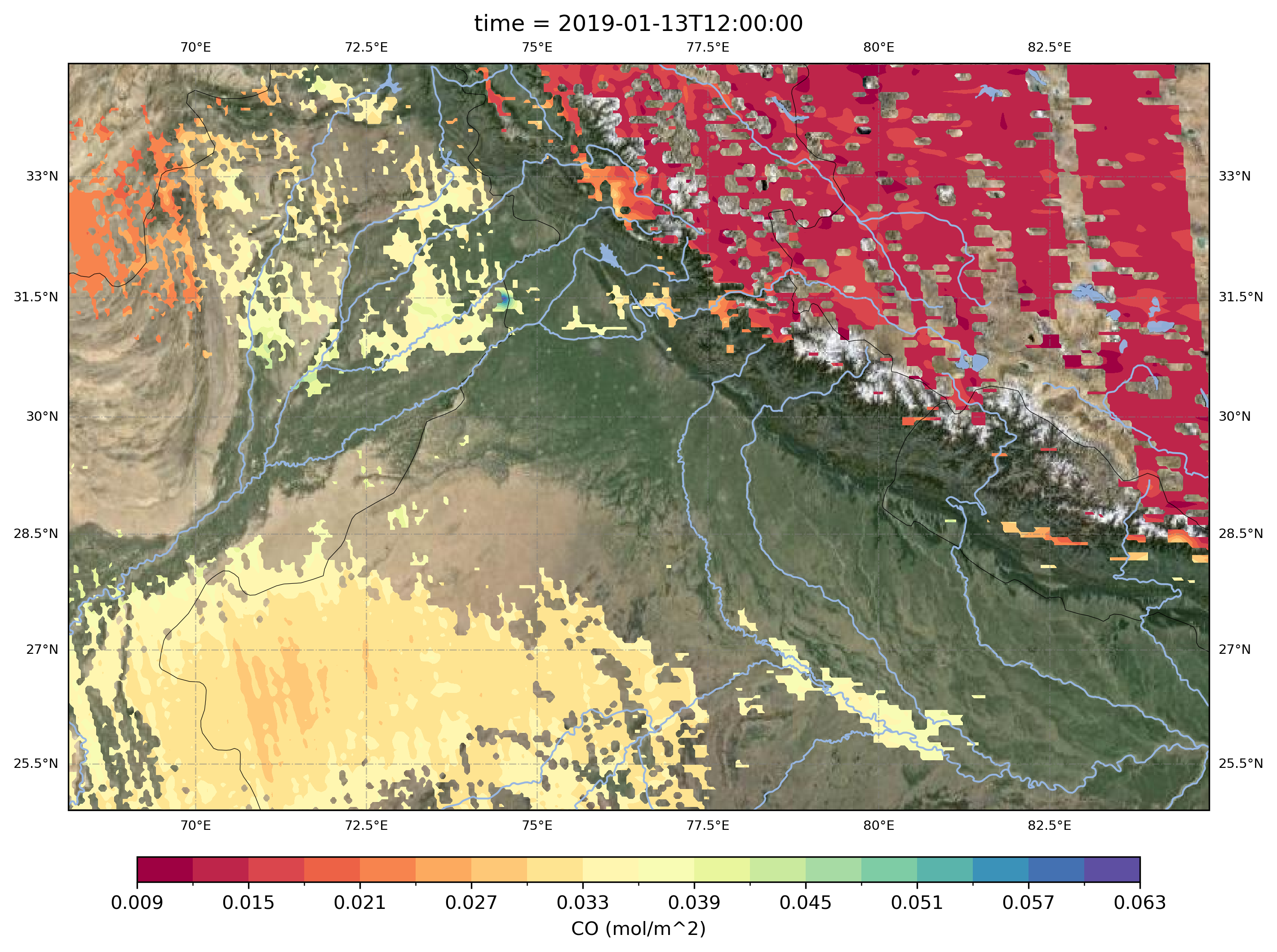
The following predictor variables were chose for training the ConvLSTM.
2.1.1 Methane – CH4
In [3]:
2.1.2 Ozone – O3
In [4]:
2.1.3 Sulphur Dioxide – SO2
In [5]:
2.1.4 Carbon Monoxide – CO
In [6]:
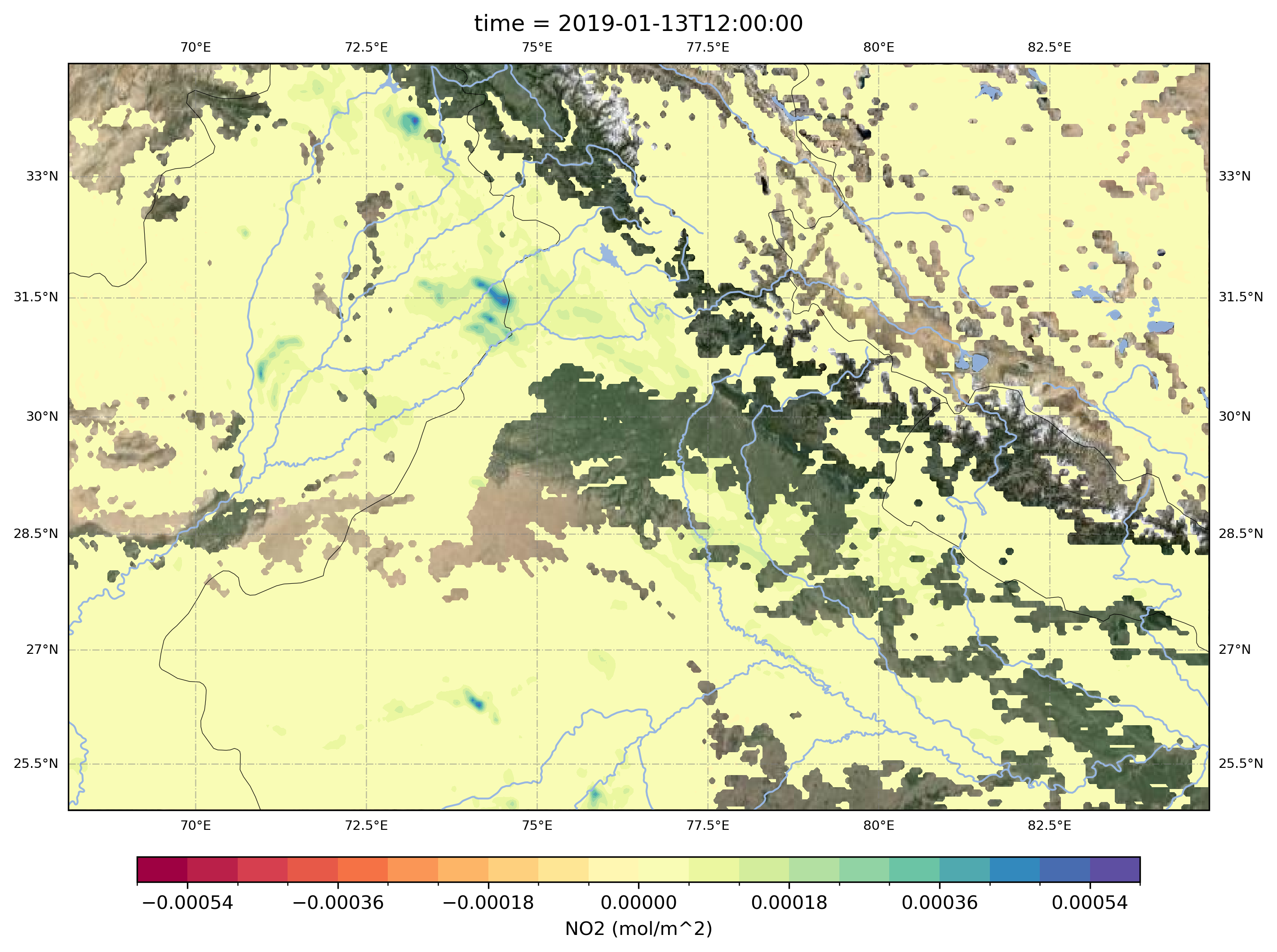
2.1.5 Nitrogen Dioxide – NO2
In [7]:
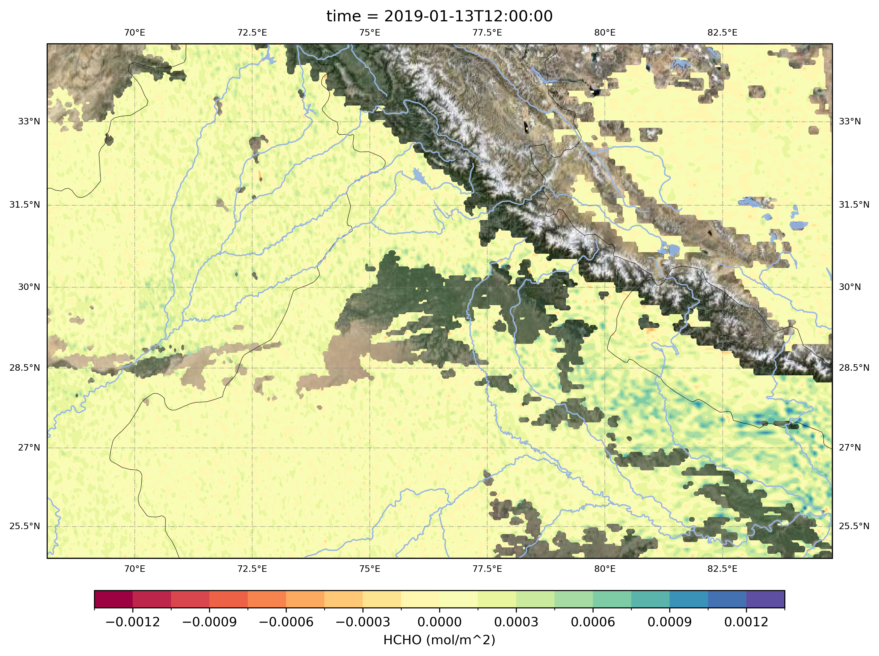
2.1.6 Formaldehyde – HCHO
In [8]:
2.2 Target variable
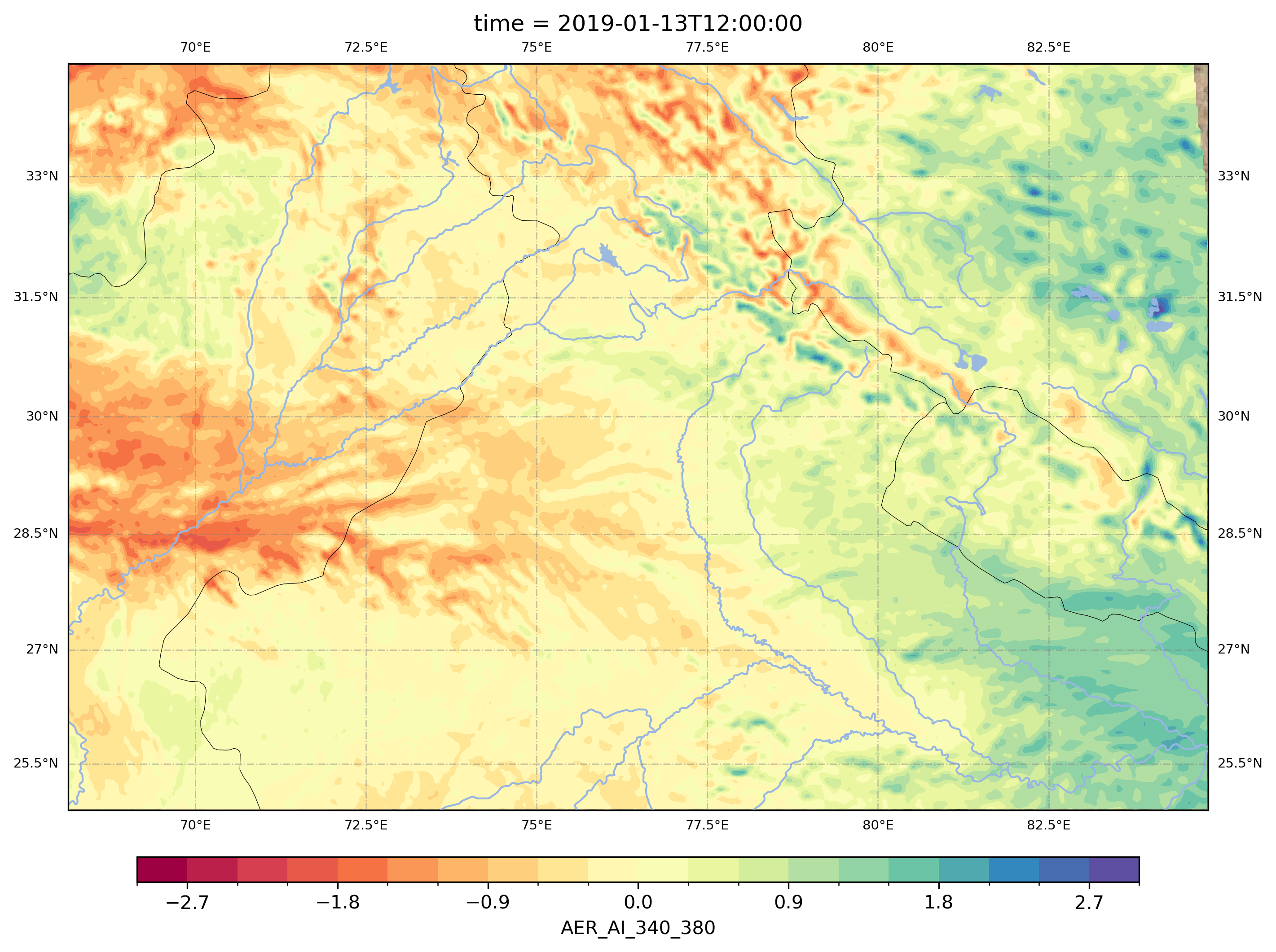
2.2.1 Aerosol Index – AI (340-380 nm)
In [9]:
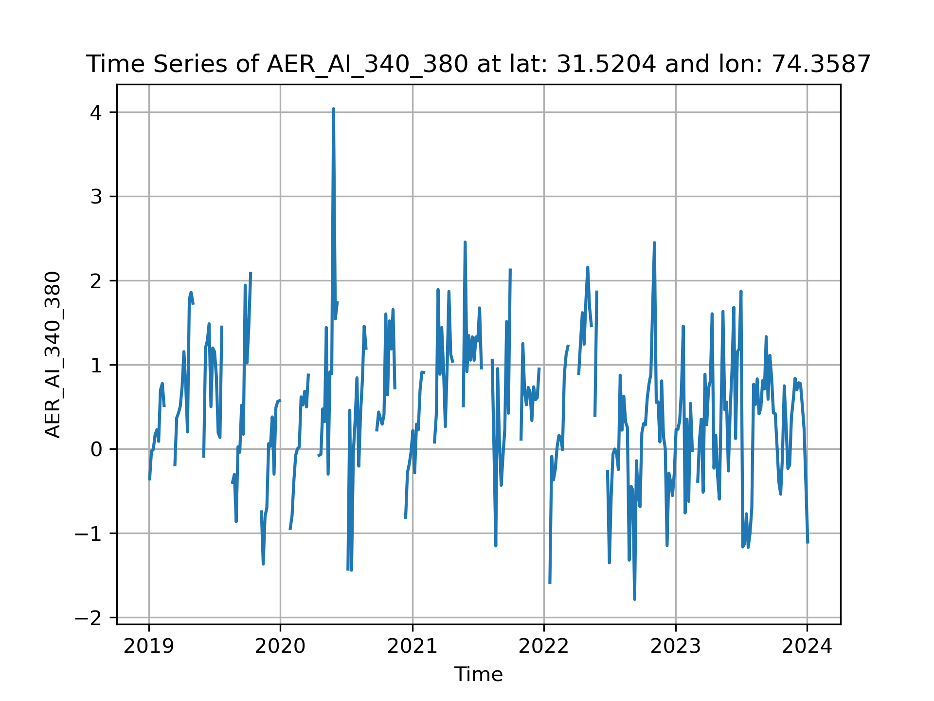
The Aerosol Index shows large variability through the year and across years.
In [10]:
3 Model Training
A Convolutional Long Short-Term Memory (ConvLSTM) model is a specialized neural network architecture that integrates the strengths of Convolutional Neural Networks (CNNs) and Long Short-Term Memory networks (LSTMs) (Luo, Liu, and Gao (2017)). This hybrid model is particularly well-suited for tasks involving spatiotemporal data, where both spatial and temporal dependencies are critical. The primary advantage of ConvLSTM models lies in their ability to simultaneously process and analyze spatial and temporal information, making them more effective for spatiotemporal tasks compared to using separate CNN and LSTM models. ConvLSTM models are used extensively in fields such as video processing, weather forecasting, and environmental monitoring, where data exhibits strong correlations across both space and time.
In [12]:
image_path = "static/convlstm.png"
Image(filename=image_path)The idea is to use the predictor variables as input to the ConvLSTM and to get the taget variable as an output.The model was trained at 50 and 100 epochs. The model was trained using the Adam optimizer with a learning rate of 0.001 and a batch size of 32.
I used the numpy (Harris et al. (2020)) python package for all the data preprocssing steps and then I used Tensorflow (Martin (2015)) and Keras (Chollet et al. (2015)) python packages for building a custom ConvLSTM. I used matplotlib (Hunter (2007)) for all plotting tasks.
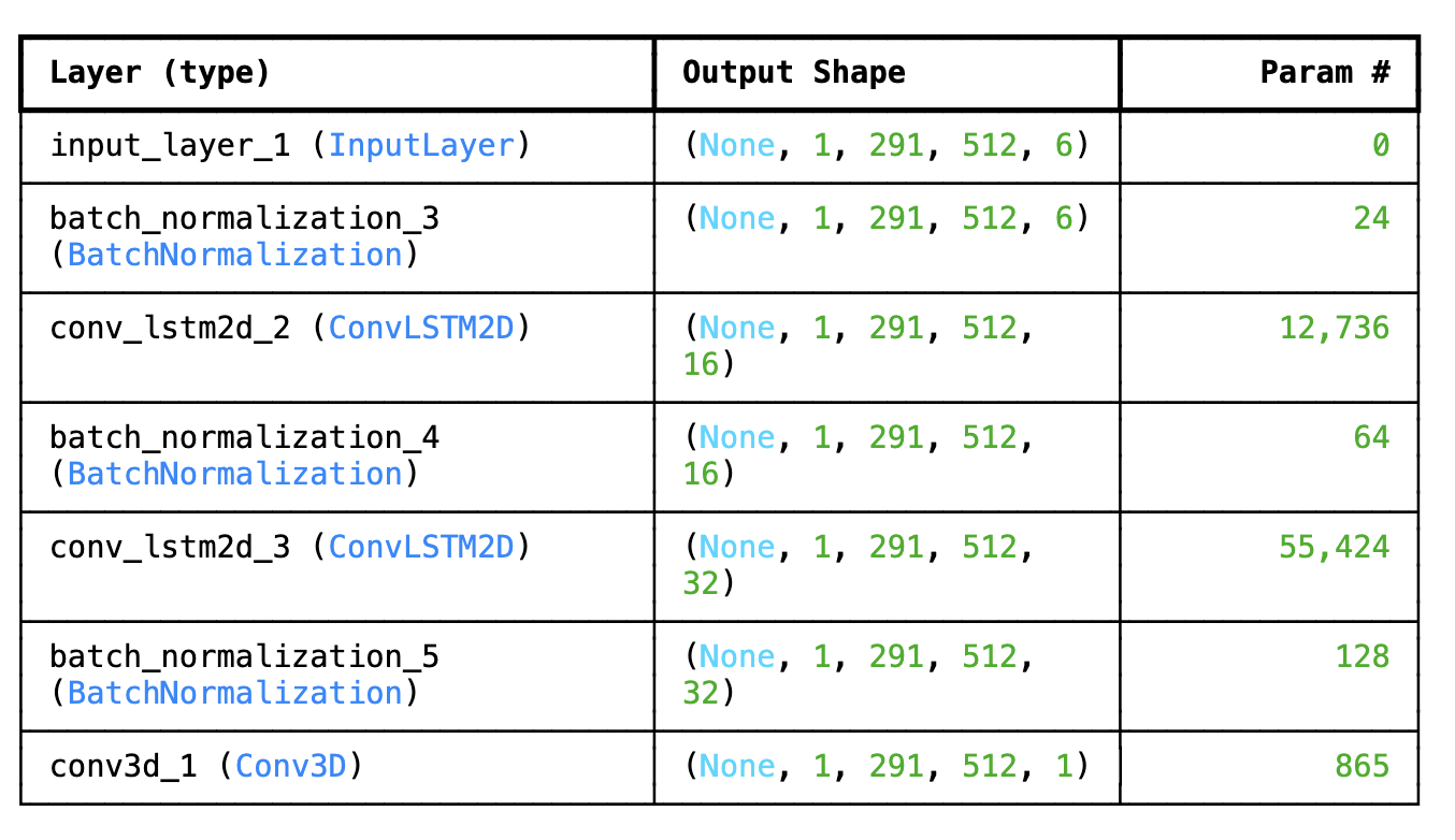
As model training required a lot of memory, the DeepESDL Jupyter Lab proved to be insufficient. Hence, I had to train the model at the Model Server Grid (MSG) Windows cluster at the Helmholtz - Center for Environmental Research (UFZ) in Leipzig, Germany Even then, the model arichtecture had to be simplified to reduce the memory requirements. The model architecture is as follows:
In [13]:
The training took approximately 4 hours for 50 epochs and 10 hours for 100 epochs.
The feature training (X_train) dataset dimesion were: (292, 1, 291, 512, 6). Here is the breakdown.
292: dates
1: time step
291: latitudes
512: longitudes
6: Features ['SO2', 'NO2', 'CH4', 'O3', 'CO', 'HCHO']
The feature testing (X_val) dataset dimesion were: (74, 1, 291, 512, 6). Here is the breakdown.
74: dates
1: time step
291: latitudes
512: longitudes
6: Features ['SO2', 'NO2', 'CH4', 'O3', 'CO', 'HCHO']
The target training (y_train) dataset dimension was: (292, 1, 291, 512, 1). Here is the breakdown.
292: dates
1: time step
291: latitudes
512: longitudes
1: Target ['AI']
The target testing (y_val) dataset dimension was: (74, 1, 291, 512, 1). Here is the breakdown.
74: dates
1: time step
291: latitudes
512: longitudes
1: Target ['AI']
3.1 Model Workflow
Here is a workflow for the provided code in smogseer.py:
A run of the code can be found in smogseer50.py and smogseer100.py.
- Import Libraries:
- Import necessary libraries such as
xarray,numpy,tensorflow,sklearn, andmatplotlib.
- Import necessary libraries such as
- Load Dataset:
- Load the dataset using
xarray.open_dataset().
- Load the dataset using
- Stack Features:
- Stack the features into a single
DataArrayand transpose to desired dimensions.
- Stack the features into a single
- Convert to NumPy Arrays:
- Convert the
DataArrayto a NumPy array.
- Convert the
- Normalize Input Data:
- Normalize the input data using
StandardScaler.
- Normalize the input data using
- Impute Missing Values in Input Data:
- Reshape the data for imputation.
- Impute missing values using
SimpleImputer. - Reshape the data back to original dimensions.
- Add Time Dimension to Input Data:
- Add an additional time dimension to the input data.
- Load Target Data:
- Load the target dataset using
xarray.open_dataset().
- Load the target dataset using
- Normalize Target Data:
- Normalize the target data using
MinMaxScaler.
- Normalize the target data using
- Impute Missing Values in Target Data:
- Reshape the target data for imputation.
- Impute missing values using
SimpleImputer. - Reshape the target data back to original dimensions.
- Ensure Target Data Shape:
- Ensure the target data shape is
(num_samples, num_timesteps, num_latitudes, num_longitudes, 1).
- Ensure the target data shape is
- Remove Samples with NaN Values:
- Identify and remove samples with NaN values in the target data.
- Verify Target Data Range:
- Ensure the target data values are within the valid range
[0, 1].
- Ensure the target data values are within the valid range
- Split Data into Training and Validation Sets:
- Split the cleaned data into training and validation sets based on a defined ratio.
- Define Model Architecture:
- Define the model architecture using
ConvLSTM2DandConv3Dlayers with appropriate activation functions and initializers. - Add batch normalization layers between LSTM layers.
- Define the model architecture using
- Compile Model:
- Compile the model with
Adamoptimizer,binary_crossentropyloss, andmean_square_erroras a metric.
- Compile the model with
- Print Model Summary:
- Print the summary of the defined model.
- Define Data Generator Class:
- Define a
DataGeneratorclass to handle large datasets efficiently.
- Define a
- Initialize Data Generators:
- Initialize training and validation data generators with a specified batch size.
- Define Callbacks for Training:
- Define callbacks for reducing learning rate, early stopping, and TensorBoard logging.
- Train the Model:
- Train the model using the data generators and defined callbacks.
- Save the Model:
- Save the trained model to a keras file .
- Load the Model:
- Load the saved model for further evaluation and prediction.
- Run Predictions on Validation Data:
- Run predictions on the validation data using the loaded model.
- Evaluate the Model:
- Evaluate the model on the validation data to obtain loss and accuracy.
- Binary Classification Threshold:
- Apply a threshold to convert predictions to binary values for classification.
- Flatten Predictions and Ground Truth:
- Flatten the predictions and ground truth data for comparison.
- Plot Comparisons and Training History:
- Define functions to plot comparisons between ground truth and predictions.
- Visualize a few samples by plotting comparisons.
- Define a function to plot training and validation loss and accuracy over epochs.
- Plot and save the training history.
To load the 50 epoch model and run predictions on the validation data, you can use the following code:
## LOAD CHECKPOINTS IF NEEDED
X_val = np.load('data/X_val.npy')
y_val = np.load('data/Y_val.npy')

# Load the model
model = load_model('smogseer50.keras')

# Run predictions on validation data
predictions = model.predict(X_val)

# Evaluate the model on validation data
val_loss, val_accuracy = model.evaluate(X_val, y_val)
print(f"Validation Loss: {val_loss}")
print(f"Validation Accuracy: {val_accuracy}")
In [3]:
## LOAD CHECKPOINTS IF NEEDED
X_val = np.load('X_val.npy')
y_val = np.load('Y_val.npy')

# Load the model
model = load_model('smogseer50.keras')

# Run predictions on validation data
predictions = model.predict(X_val)

# Evaluate the model on validation data
val_loss, val_accuracy = model.evaluate(X_val, y_val)
print(f"Validation Loss: {val_loss}")
print(f"Validation Accuracy: {val_accuracy}")
3/3 ━━━━━━━━━━━━━━━━━━━━ 7s 693ms/step
3/3 ━━━━━━━━━━━━━━━━━━━━ 3s 432ms/step - loss: 0.3992 - mean_squared_error: 0.0016
Validation Loss: 0.39958614110946655
Validation Accuracy: 0.0018263210076838732To load the 100 epoch model and run predictions on the validation data, you can use the following code:
## LOAD CHECKPOINTS IF NEEDED
X_val = np.load('data/X_val.npy')
y_val = np.load('data/Y_val.npy')

# Load the model
model = load_model('smogseer100.keras')

# Run predictions on validation data
predictions = model.predict(X_val)

# Evaluate the model on validation data
val_loss, val_accuracy = model.evaluate(X_val, y_val)
print(f"Validation Loss: {val_loss}")
print(f"Validation Accuracy: {val_accuracy}")
In [4]:
# Load the model
model = load_model('smogseer100.keras')

# Run predictions on validation data
predictions = model.predict(X_val)

# Evaluate the model on validation data
val_loss, val_accuracy = model.evaluate(X_val, y_val)
print(f"Validation Loss: {val_loss}")
print(f"Validation Accuracy: {val_accuracy}")
3/3 ━━━━━━━━━━━━━━━━━━━━ 3s 632ms/step
3/3 ━━━━━━━━━━━━━━━━━━━━ 3s 423ms/step - loss: 0.4003 - mean_squared_error: 0.0019
Validation Loss: 0.40102294087409973
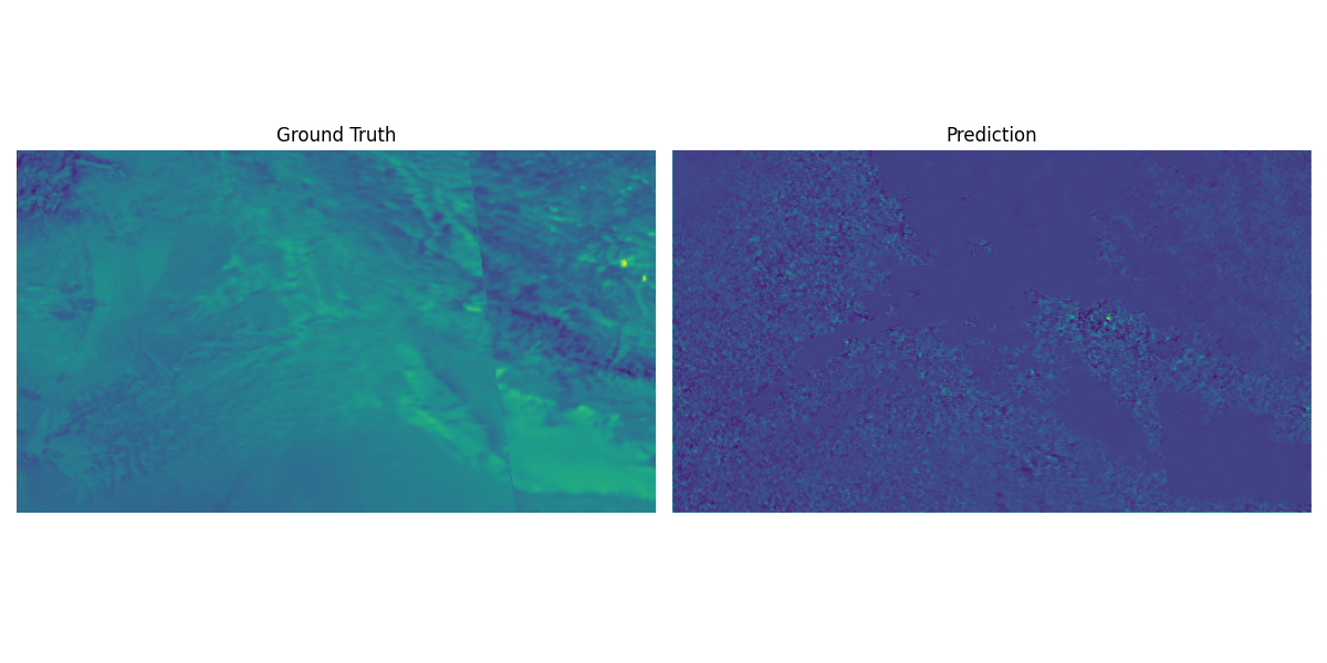
Validation Accuracy: 0.0022550118155777454The images were converted to a GIF. The ground truth for the same time period was also visualised. The GIFs can be see side by side here:
In [22]:
The model prediction and gorund truth data were visualised side by side for 5 timesteps, which is 25 days. These images can be found in the static folder in the repository.
An example:
In [21]:
image_path = "static/comparison.gif"
Image(filename=image_path)
<IPython.core.display.Image object>4 Evaluation
The evaluation metrics used in Smogseer are: 1. Binary Crossentropy Loss, 2. Mean Squared Error.
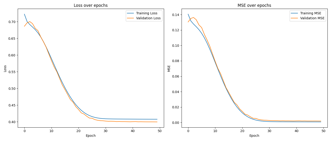
Here is what the evaluation metrics look like for the 50 epochs model:
In [16]:
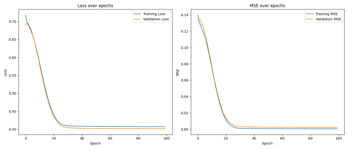
And here is what the evaluation metrics look like for the 100 epochs model:
In [17]:
5 Conclusion
5.1 Loss over Epochs
Training Loss (Blue Line):
- The training loss starts at around 0.70 and decreases steadily as the number of epochs increases.
- It shows a continuous decline, indicating that the model is learning from the training data and improving its performance.
Validation Loss (Orange Line):
- The validation loss starts slightly higher than the training loss, which is typical.
- It follows a similar declining trend as the training loss.
- The validation loss closely tracks the training loss, which suggests that the model is generalizing well to the validation data without overfitting.
5.2 MSE over Epochs
Training MSE (Blue Line):
- The training MSE starts at a high value and decreases steadily, similar to the training loss.
- This decrease indicates that the model’s predictions are becoming closer to the actual target values as training progresses.
Validation MSE (Orange Line):
- The validation MSE also starts high and decreases over the epochs.
- It tracks the training MSE closely, reinforcing that the model’s performance on unseen data is improving without significant overfitting.
5.3 Key Observations
- Steady Decrease: Both the loss and MSE for training and validation datasets are steadily decreasing, which is a positive sign that the model is learning effectively.
- No Overfitting: Since the validation loss and MSE closely follow the training loss and MSE without diverging, it indicates that there is no significant overfitting.
- Plateauing: Both training and validation loss/MSE curves start to plateau after about 30 epochs. This suggests that further training may not significantly improve the model’s performance.
5.4 Recommendations
- Early Stopping: Implement early stopping in future training runs to stop training when the validation loss stops improving, saving computational resources and potentially preventing overfitting.
- Learning Rate: If you observe the model’s performance plateauing, consider decreasing the learning rate to allow for finer adjustments to the weights.
- Model architecture: Experiment with different model architectures, hyperparameters, or additional features to improve the model’s predictive performance.
